1 Visualization

View solutions

Statistics can be divided into two broad categories: descriptive statistics, which describe or summarise data, and inferential statistics, which allow us to infer something about a population from a sample.

This session focuses on descriptive statistics: how to appropriately display and summarise. You already know several techniques for displaying data (e.g., bar charts, histograms, scatter plots). When and how to use these techniques is one focus of today.

There are two critical purposes of data visualization:

Getting a ‘gut’ feel for your data. Examining data graphically enables you to identify any outliers (suspicious observations which could be errors). It will also help you to select the most appropriate inferential statistical model (more on this later).
Communicating your results. Focus on clarity, drawing attention to the most interesting aspects of your data. Graphics that are confusing, either through a lack of detail (e.g. no labels) or that contain too much information will fail in this central objective.

As you create graphics, keep in mind that they may be viewed on different machines, in grey scale, or by colour-blind or visually impaired readers. Colour scales such as those available from ColorBrewer or viridis are designed with this in mind.

1.1 R Review

We very briefly review key basics of R here. See R Basics for a more comprehensive review.

It’s best practice to load necessary packages at the top of your document. Remember, packages need to be installed once per machine, but loaded in each R session.

To install a package, either click the link in the yellow banner at the top of your script (RStudio usually does this when needed), or run:

install.packages("tidyverse")
install.packages("cowplot")

You will likely not need to do that again this semester! However, you will need to use library(packageName) each time you open R.

library(tidyverse)
library(readxl) # installed with tidyverse, but not loaded in library(tidyverse)
library(cowplot)
set.seed(2026) # for fully reproducible code
theme_set(theme_classic()) # plotting theme

1.2 Basic data exploration

1.2.1 Object structure

We will mostly work with dataframes. A data.frame is a 2D rectangular object with columns and rows. In a tidy dataset, each row represents an ‘observation’ and each column represents a ‘variable’. R (and often packages) contains several built-in dataframes, bundled into the datasets package which is automatically loaded.

# functions for basic details of objects
str(penguins) # structure overview
glimpse(penguins) # slightly different overview
names(penguins) # column names
head(penguins) # first few rows

Functions have arguments, which let you control their settings. They typically have defaults, which you can see in the help page. For example, head() shows the first 6 rows by default (?head: note n = 6L). Specify the argument to adjust the behaviour:

head(penguins, n=2)

  species    island bill_len bill_dep flipper_len body_mass    sex year
1  Adelie Torgersen     39.1     18.7         181      3750   male 2007
2  Adelie Torgersen     39.5     17.4         186      3800 female 2007

tail(penguins, n=2)

      species island bill_len bill_dep flipper_len body_mass    sex year
343 Chinstrap  Dream     50.8     19.0         210      4100   male 2009
344 Chinstrap  Dream     50.2     18.7         198      3775 female 2009

# what are the last 10 rows?

Function arguments do not need to be named if they are listed in the order given in the help documentation. For example, head(penguins, 2) will do exactly the same thing as head(x=penguins, n=2).

1.2.2 Subsetting, renaming, and rearranging

There are several ways to access subsets of a data.frame:

Use data_df$columnName to extract a single column
Use data_df[rows,columns] to extract a block

penguins$bill_len # whole column

penguins[1, 3] # row 1, column 3

[1] 39.1

penguins[1:5, 3] # rows 1-5, column 3

[1] 39.1 39.5 40.3   NA 36.7

penguins[2:4, ] # leaving the 'columns' blank will return all columns

  species    island bill_len bill_dep flipper_len body_mass    sex year
2  Adelie Torgersen     39.5     17.4         186      3800 female 2007
3  Adelie Torgersen     40.3     18.0         195      3250 female 2007
4  Adelie Torgersen       NA       NA          NA        NA   <NA> 2007

We can also change column names. For illustration, let’s make a copy of the data.frame to do that.

penguins_alt <- penguins 
names(penguins_alt)

[1] "species"     "island"      "bill_len"    "bill_dep"    "flipper_len"
[6] "body_mass"   "sex"         "year"

names(penguins_alt)[1] <- "species_name" # change first column name
names(penguins_alt)

[1] "species_name" "island"       "bill_len"     "bill_dep"     "flipper_len" 
[6] "body_mass"    "sex"          "year"

Create a new column by specifying the name with df$colName and assigning a vector.

penguins_alt$bill_area <- penguins_alt$bill_dep * penguins_alt$bill_len
head(penguins_alt, 2)

  species_name    island bill_len bill_dep flipper_len body_mass    sex year
1       Adelie Torgersen     39.1     18.7         181      3750   male 2007
2       Adelie Torgersen     39.5     17.4         186      3800 female 2007
  bill_area
1    731.17
2    687.30

Recall that you must assign the results of an operation (<-) to save it. For example, running penguins_alt[, 2:1] will display the results, but penguins_alt <- penguins_alt[, 2:1] will overwrite penguins_alt in your R environment.

You can also subset based on criteria. Say we only want rows with observations from 2009:

penguins_2009 <- penguins_alt[penguins_alt$year == 2009, ]

It is always good to check that you’ve done what you think you’ve done:

nrow(penguins_2009)

[1] 120

head(penguins_2009, 2)

    species_name island bill_len bill_dep flipper_len body_mass    sex year
101       Adelie Biscoe       35     17.9         192      3725 female 2009
102       Adelie Biscoe       41     20.0         203      4725   male 2009
    bill_area
101     626.5
102     820.0

count(penguins_alt, year)

count(penguins_2009, year)

  year   n
1 2009 120

1.2.3 NAs and summary

When you import data, you should check for missing values. These are represented as NA.

We can check each element of a vector using is.na(), which will return TRUE if an element is NA, and FALSE if an element is not NA.

is.na(penguins_alt$sex)

R converts logical values (i.e., TRUE/FALSE) to numeric (i.e., 1/0) automatically, allowing convenient summaries:

sum(is.na(penguins_alt$sex)) # how many are NA?

[1] 11

mean(is.na(penguins_alt$sex)) # what proportion are NA?

[1] 0.03197674

Another very useful check is summary():

summary(penguins_alt)

    species_name       island       bill_len        bill_dep    
 Adelie   :152   Biscoe   :168   Min.   :32.10   Min.   :13.10  
 Chinstrap: 68   Dream    :124   1st Qu.:39.23   1st Qu.:15.60  
 Gentoo   :124   Torgersen: 52   Median :44.45   Median :17.30  
                                 Mean   :43.92   Mean   :17.15  
                                 3rd Qu.:48.50   3rd Qu.:18.70  
                                 Max.   :59.60   Max.   :21.50  
                                 NA's   :2       NA's   :2      
  flipper_len      body_mass        sex           year        bill_area     
 Min.   :172.0   Min.   :2700   female:165   Min.   :2007   Min.   : 497.6  
 1st Qu.:190.0   1st Qu.:3550   male  :168   1st Qu.:2007   1st Qu.: 667.7  
 Median :197.0   Median :4050   NA's  : 11   Median :2008   Median : 730.8  
 Mean   :200.9   Mean   :4202                Mean   :2008   Mean   : 750.8  
 3rd Qu.:213.0   3rd Qu.:4750                3rd Qu.:2009   3rd Qu.: 807.2  
 Max.   :231.0   Max.   :6300                Max.   :2009   Max.   :1127.4  
 NA's   :2       NA's   :2                                  NA's   :2

summary(penguins_alt)

Once you are confident that your data.frame looks sensible, that it contains the data you expect, and that the data types are correct, you can start to explore and summarise your data.

There are many graphical methods for data exploration. The appropriate method depends on the nature of the data and what you wish to communicate to the reader.

1.3 Graphical methods for displaying data

Always keep in mind that the primary reason for data visualization is to communicate concisely and accurately to your reader. Graphics should be clear, concise and easy to understand.

Real data is usually complex, and creating effective figures takes careful thought and often many revisions.

We will primarily use the ggplot2 package because it is more straightforward in many ways. It loads when you run library(tidyverse). However, we will also note equivalent base R functions from time to time.

1.3.1 Scatter plots

Scatter plots display two continuous variables against each other. They are commonly used for analyses like correlation or linear regression.

With ggplot2:

ggplot(penguins_alt, aes(x=body_mass, y=bill_len)) + 
  geom_point() + 
  labs(x="Body mass (g)", 
       y="Bill length (mm)",
       title="Bill length increases with body mass")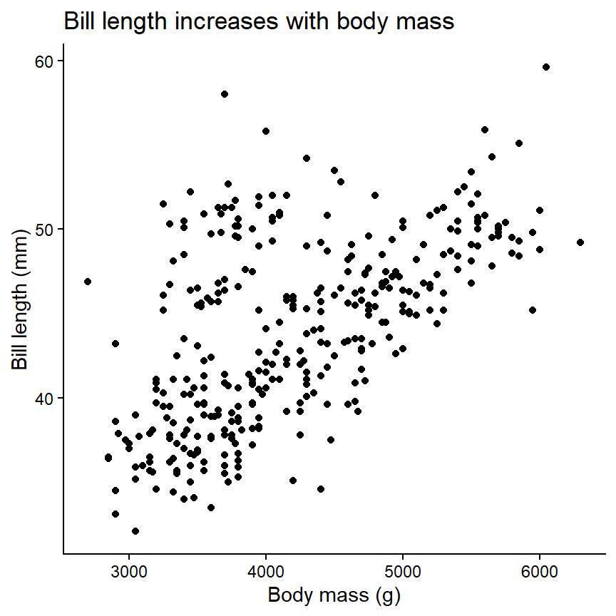

The ggplot() function takes the dataframe as the first argument. The plot aesthetics are specified with aes(), such that variables (=columns) are mapped to plot aesthetics. Then, layers are added using geom_*(). Additional functions can be ‘added’ to further modify the plot. See a comprehensive list in the ggplot2 manual.

Once you understand the basic structure, it becomes easy to create more interesting figures:

ggplot(penguins_alt, aes(x=body_mass, y=bill_len, colour=species_name)) + 
  geom_point() + 
  geom_line(stat="smooth", method="lm") +
  scale_colour_brewer("Species", palette="Dark2") +
  labs(x="Body mass (g)", 
       y="Bill length (mm)",
       title="Bill length increases with body mass")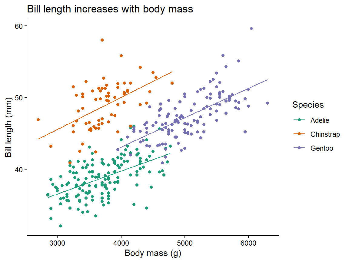

With base R, the plot() function will create a scatter plot if given two numeric variables. There are two options for specifying the variables.

Using data_df with columns x and y, the same plot can be created with either syntax:

data_df <- data.frame(x=1:3, y=4:6)
plot(data_df$x, data_df$y) # two vectors: x, y
plot(y ~ x, data=data_df) # columns in dataframe: formula y ~ x

There are many options for modifying the output of plot(), but it is clunkier compared to ggplot2.

Q. 1.1

With the penguins dataset, plot bill length by body mass for only Chinstrap penguins. Make sure the plot is fully labelled.

View solution

ggplot(penguins[penguins$species=="Chinstrap",], aes(body_mass, bill_len)) +
  geom_point() + 
  labs(x="Body mass (g)", 
       y="Bill length (mm)",
       title="Chinstrap penguins")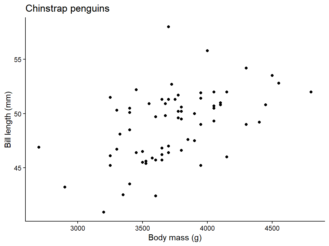

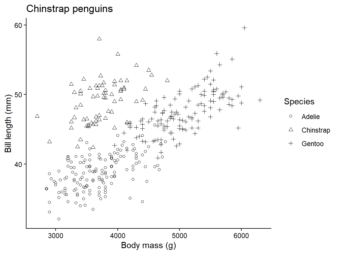
Figure 1.1: Chinstrap penguin allometrics.

Q. 1.2

Using ggplot(), create a figure where each species is a different shape. See the Aesthetics section in ?geom_point for help.

1.3.2 Boxplots

Box plots are used to summarise a continuous variable by levels of a factor.

Explore the data.frame using the strategies covered above. Which variables are categorical? Which are continuous?

'data.frame':   344 obs. of  8 variables:
 $ species    : Factor w/ 3 levels "Adelie","Chinstrap",..: 1 1 1 1 1 1 1 1 1 1 ...
 $ island     : Factor w/ 3 levels "Biscoe","Dream",..: 3 3 3 3 3 3 3 3 3 3 ...
 $ bill_len   : num  39.1 39.5 40.3 NA 36.7 39.3 38.9 39.2 34.1 42 ...
 $ bill_dep   : num  18.7 17.4 18 NA 19.3 20.6 17.8 19.6 18.1 20.2 ...
 $ flipper_len: int  181 186 195 NA 193 190 181 195 193 190 ...
 $ body_mass  : int  3750 3800 3250 NA 3450 3650 3625 4675 3475 4250 ...
 $ sex        : Factor w/ 2 levels "female","male": 2 1 1 NA 1 2 1 2 NA NA ...
 $ year       : int  2007 2007 2007 2007 2007 2007 2007 2007 2007 2007 ...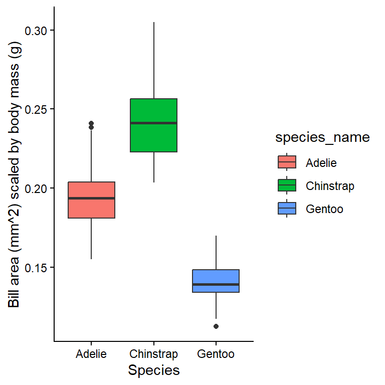

Figure 1.3: Boxplot showing bill area by species

?geom_boxplot
# See examples at bottom of the help page

Q. 1.3

Reproduce the plot shown in Figure 1.3.

View solution

ggplot(penguins_alt, aes(species_name, bill_area/body_mass, fill=species_name)) + 
  geom_boxplot() +
  labs(x="Species", 
       y="Bill area (mm^2) scaled by body mass (g)")

Q. 1.4

Use ?boxplot.stats to investigate what the box and whiskers actually represent.

In base R, use boxplot(y ~ x, data=dataframe) to create a boxplot.

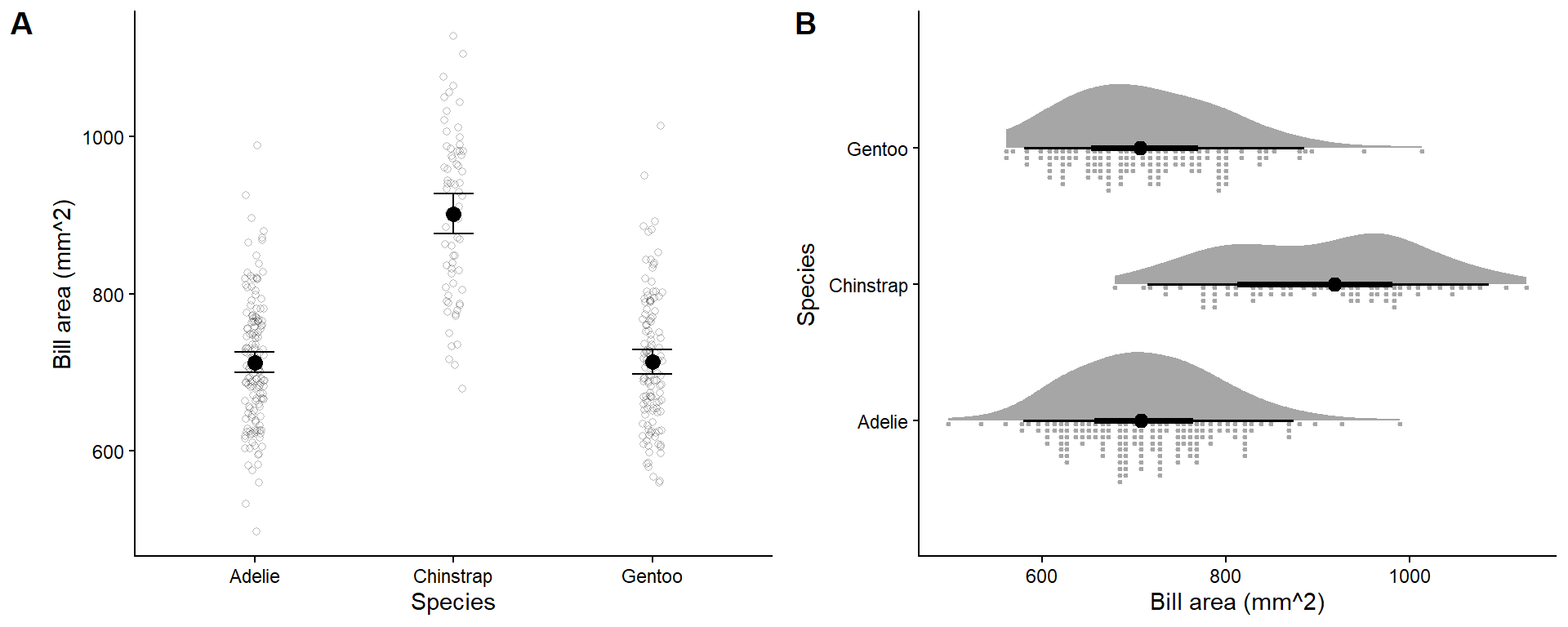
Note that box plots are not the most visually intuitive, since smaller box areas correspond with more observations. Packages like ggplot2 (and extensions) make alternatives like those in Figure 1.4 simple to produce. We will cover some of these later.

Figure 1.4: Alternatives to boxplots. (A) Strip plot which shows all data along with means and 2 standard errors. (B) Rain cloud plot showing data distributions along with medians with middle 50% and 95%.

1.3.3 Line plots

Line plots are most often seen in timeseries plots with time on the x-axis and the response on the y-axis. Line plots involve joining points with a line, which indicates that you have made assumptions about the value of the response variable between successive measurements.

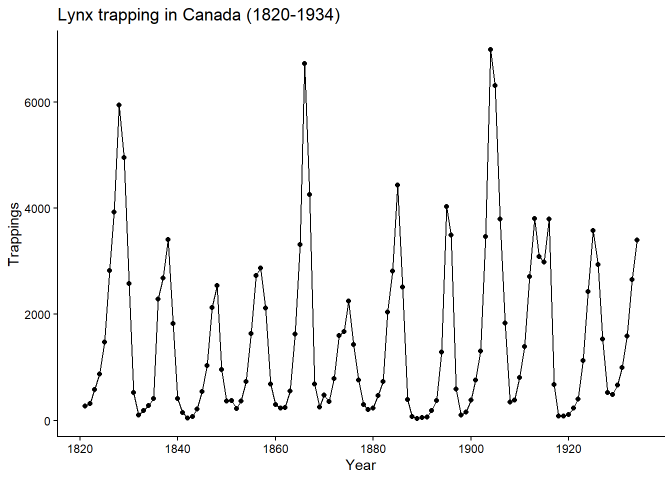
We will examine these plots using the dataset lynx, which consists of the number of Canadian lynx pelts sold per year between 1821 - 1934. It is a ‘classic’ dataset as it shows a cyclical ‘boom-and-bust’ lynx population (demonstrating predator-prey interactions).

First, we will create a variable Year.

str(lynx)

 Time-Series [1:114] from 1821 to 1934: 269 321 585 871 1475 ...

str(lynx)
lynx_df <- as.data.frame(lynx) 
str(lynx_df) 
lynx_df$Year <- seq(from=1821, to=1934, by=1)
lynx_df$Trappings <- as.numeric(lynx_df$x) # Time-Series is complicated.
str(lynx_df)
head(lynx_df, 2)

In R, we use functions to perform actions on objects. Functions have arguments, taking the form functionName(arg1=..., arg2=...). If you do not name the arguments, the function will assume that you are listing the arguments in order. See the help file for a function with ? to see the argument order (e.g., ?seq).

Q. 1.5

Using seq(), write a piece of code which generates odd numbers between 1 and 20. Try with and without naming the arguments.

View solution

seq(from=1, to=20, by=2)
seq(1, 20, 2)

Q. 1.6

Using ggplot(), produce a line plot similar to Figure 1.5.

Figure 1.5: The number of lynx trapped in Canada (1820-1934)

View solution

ggplot(lynx_df, aes(Year, Trappings)) +
  geom_point() +
  geom_line() + 
  labs(title="Lynx trapping in Canada (1820-1934)")

In base R, use plot(y ~ x, data=dataframe, type='b') to make plots with both points and lines, or type='l' for just lines.

Q. 1.7

Create a plot that shows the log-transformed number of trappings from only 1850 to 1900.

View solution

ggplot(lynx_df[lynx_df$Year >= 1850 & lynx_df$Year <= 1900, ], 
       aes(Year, log(Trappings))) +
  geom_point() +
  geom_line() + 
  labs(title="Lynx trapping in Canada (1850-1900)")

Alternatively (and better, in this case) is to modify the axis rather than the variable.

ggplot(lynx_df[lynx_df$Year >= 1850 & lynx_df$Year <= 1900, ], 
       aes(Year, Trappings)) +
  geom_point() +
  geom_line() + 
  scale_y_log10() +
  guides(y="axis_logticks") +
  labs(title="Lynx trapping in Canada (1850-1900)")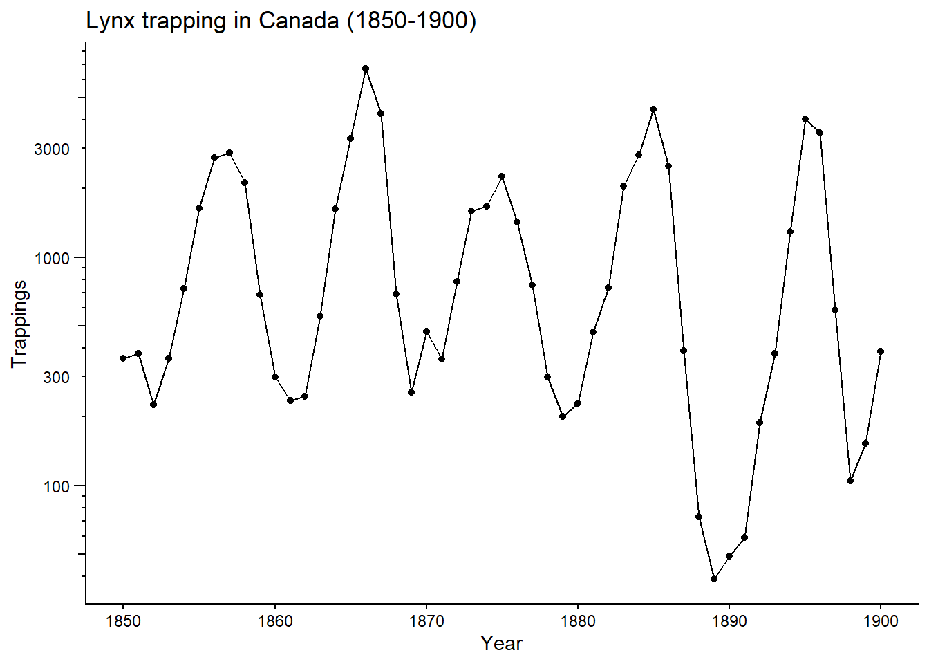

1.3.4 Histograms

Histograms illustrate the distribution of continuous data. In histograms the bars are adjacent (no gap). This indicates that the underlying values are continuous rather than discrete.

ggplot(lynx_df, aes(Trappings)) + # specify x-axis, bun not y-axis
  geom_histogram(colour="grey30", fill="grey90") + 
  labs(x="Trapped lynx per year", 
       title="Lynx trapping")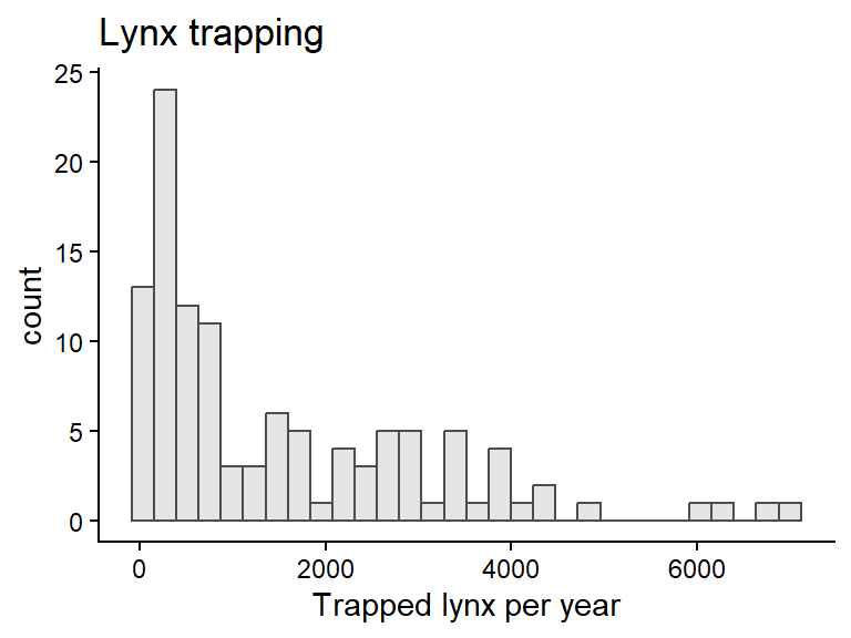

Figure 1.6: Lynx pelts per year with default settings.

Q. 1.8

What conclusions do you draw from this plot? Which range of values was most common across years?

Be aware that histograms can be quite sensitive to the number of bins, and you should explore different options. You can set the number of bins with bins=... or specific values of break points with breaks=....

To make a multi-panel figure with ggplot, use the plot_grid() function in the cowplot package.

library(cowplot)
pA <- ggplot(lynx_df, aes(Trappings)) +
  geom_histogram(colour="grey30", fill="grey90", 
                 bins=5) + 
  labs(x="Trapped lynx per year", 
       title="Lynx trapping")
pB <- ggplot(lynx_df, aes(Trappings)) +
  geom_histogram(colour="grey30", fill="grey90", 
                 breaks=c(0, 500, 1000, 2000, 5000, 10000)) + 
  labs(x="Trapped lynx per year", 
       title="Lynx trapping")
plot_grid(pA, pB, nrow=1, labels="AUTO")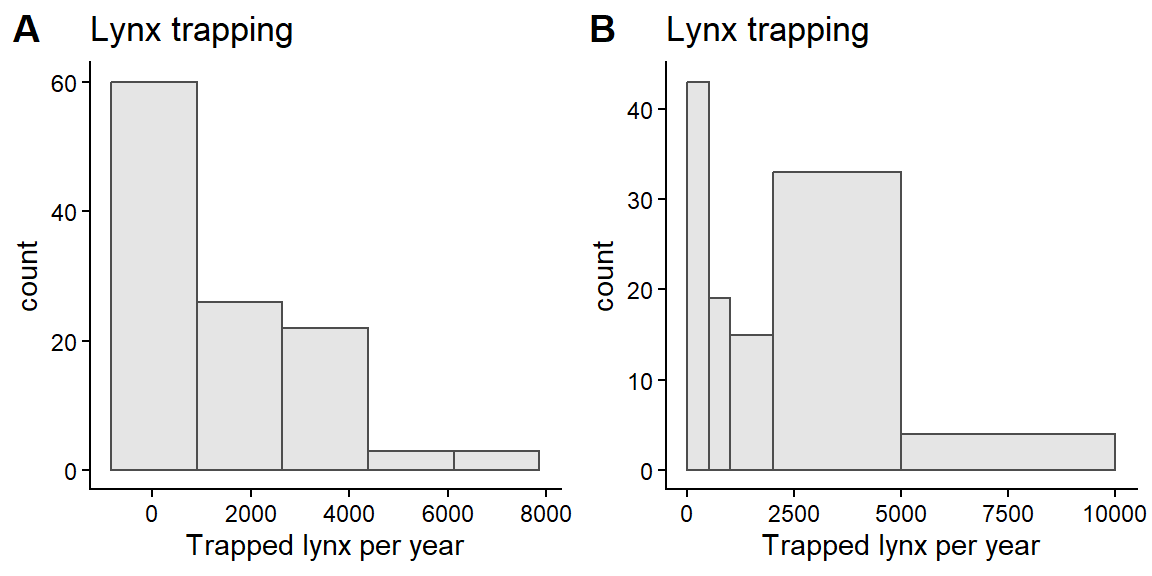

Figure 1.7: Lynx pelts per year with breaks=5 (left) and a vector of breaks (right).

Code (bonus)

pA <- ggplot(lynx_df, aes(Trappings)) +
  geom_histogram(colour="grey30", fill="grey90", 
                 breaks=seq(0, 10000, by=100)) + 
  labs(x="Trapped lynx per year")
pB <- ggplot(lynx_df, aes(Trappings)) +
  geom_histogram(colour="grey30", fill="grey90", 
                 breaks=seq(0, 10000, by=500)) + 
  labs(x="Trapped lynx per year")
pC <- ggplot(lynx_df, aes(Trappings)) +
  geom_histogram(colour="grey30", fill="grey90", 
                 breaks=seq(0, 10000, by=1000)) + 
  labs(x="Trapped lynx per year")
pD <- ggplot(lynx_df, aes(Trappings)) +
  geom_histogram(colour="grey30", fill="grey90", 
                 breaks=seq(0, 10000, by=2000)) + 
  labs(x="Trapped lynx per year")
plot_grid(pA, pB, pC, pD, nrow=2, ncol=2,
          align="hv", axis="tblr", labels="AUTO")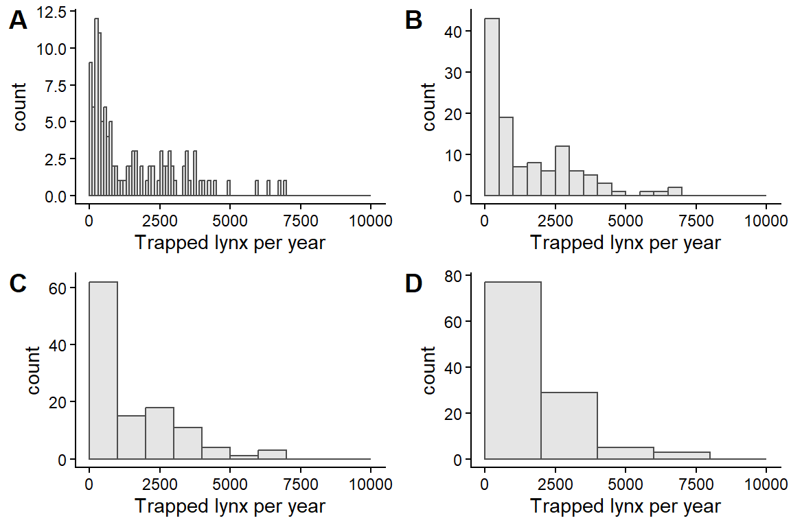

Figure 1.8: Histograms of lynx pelts per year with breaks every (A) 100, (B) 500, (C) 1,000, or (D) 2,000.

Which of these plots is the most useful? There is no definitive answer, but the first is very busy and the last fails to show relevant detail near 0. Bin widths of 500-1000 communicate the patterns most clearly.

Generally, 5-15 breaks usually work well.

In base R, use hist(dataframe$column).

1.3.5 Bar graphs

Bar graphs are used to plot counts of categorical or discrete variables. We’ll be using the islands dataset which is a named vector of island areas.

Many objects in R can have row names. However, converting between data types may lose this information. Consequently, it is better practice to store relevant information in a column. Nevertheless, there are occasions where this is useful and you may come across datasets with data stored as row names.

Working with data involves a lot of time spent tidying the datasets: cleaning, checking, and reshaping into useful formats. We will cover a more modern set of methods for this later in the course using the tidyverse package. For now, we’ll stay with base R. First, we need to tidy the islands data.

str(islands) # this is a named numeric vector
head(islands)

# convert to a dataframe
islands_df <- as.data.frame(islands) 
head(islands_df, 2)
str(islands_df) # rownames are not shown!

# put the row names into a new column
islands_df$LandMass <- row.names(islands_df) 
head(islands_df, 2)

           islands   LandMass
Africa       11506     Africa
Antarctica    5500 Antarctica

# set row names to the row number
row.names(islands_df) <- 1:nrow(islands_df) 
names(islands_df)[1] <- "Area" 
head(islands_df, 2)

   Area   LandMass
1 11506     Africa
2  5500 Antarctica

An initial attempt at a barplot makes a terrible figure.

ggplot(islands_df, aes(LandMass, Area)) + 
  geom_bar(stat="identity") # 'identity' means it won't calculate any summaries

Figure 1.9: Island areas with barplot defaults

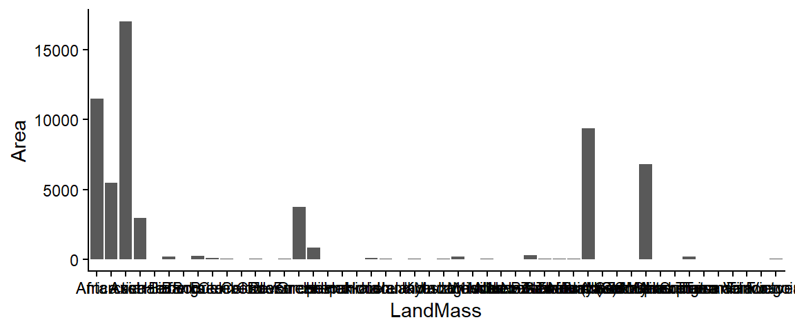
The whole dataset includes a lot of very small areas, so let’s cut it down to just the 10 largest. We also want to order the land masses by area in our plot.

We will use the arrange() function to order our dataframe, and then use scale_x_discrete() to specify the breaks in the desired order.

islands_df <- arrange(islands_df, desc(Area)) # desc() makes it largest to smallest

ggplot(islands_df[1:10,], aes(LandMass, Area)) + 
  geom_bar(stat="identity") +
  scale_x_discrete(limits=islands_df$LandMass[1:10])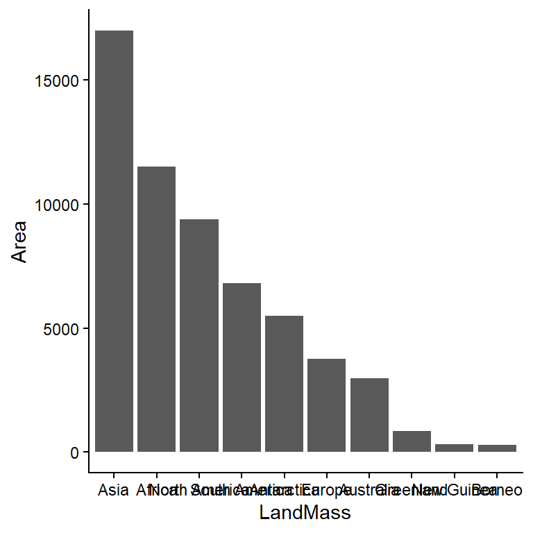

It would be more effective sideways:

ggplot(islands_df[1:10,], aes(Area, LandMass)) + 
  geom_bar(stat="identity") +
  scale_y_discrete(limits=islands_df$LandMass[10:1]) +
  labs(x="Land mass", 
       y="Area (km^2)")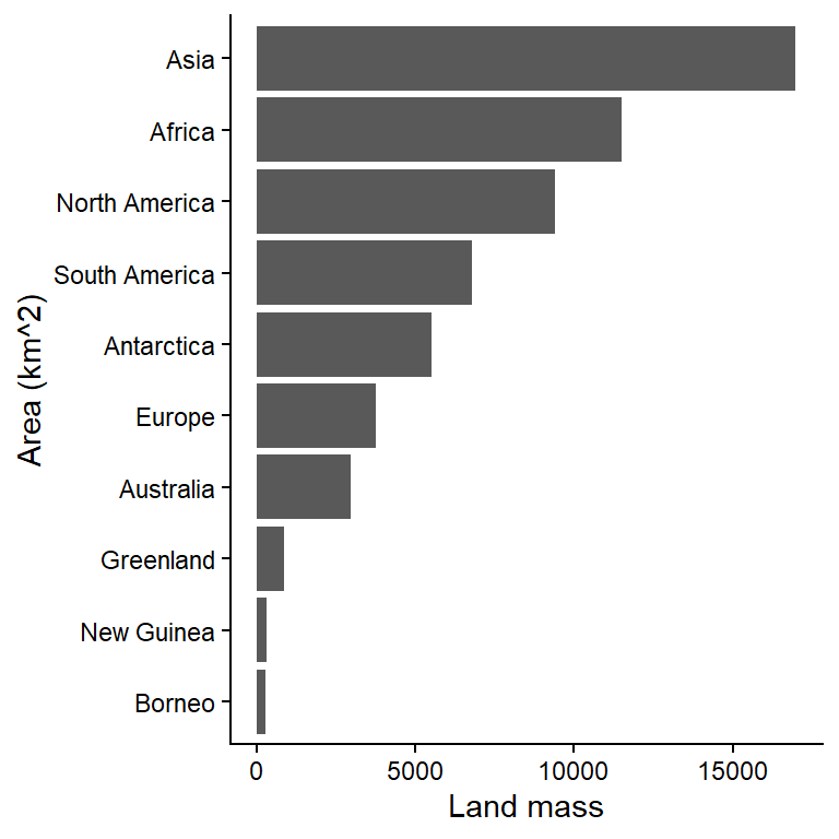

Figure 1.11: Finally! Did you know Antarctica is bigger than Europe?

Data visualization is an iterative process with lots of trial and error to find a plot that communicates the message within the data well.

1.4 Summary statistics

You will often need to summarise your data before you present it. Data summaries are usually contained in tables and they can sometimes replace graphics (e.g., where the data is relatively simple or where individual precise values are important). There are many types of summary statistics. Here we are concerned with central tendency and variability.

Q. 1.9

What are the three main measures of central tendency?

Q. 1.10

What are three measures of variability?

The most appropriate metrics of central tendency or variability will depend on your data. Another summary statistic that you might include is sample size. R is very good at producing summary statistics, and there are myriad ways to produce them.

Often you’ll wish to summarise your data across levels of a certain factor, such as levels of a certain treatment. More complex summaries can be made using the dplyr package. We’ll go into more detail later on some of the very powerful ways this package (and others in the tidyverse) can be used.

We’ll use the built-in dataset InsectSprays. Viewing your raw data can be an important check as well. You can open a spreadsheet-style viewer in R using View(YourDataFrame) or by clicking on the icon in the Environment pane.

str(InsectSprays)

'data.frame':   72 obs. of  2 variables:
 $ count: num  10 7 20 14 14 12 10 23 17 20 ...
 $ spray: Factor w/ 6 levels "A","B","C","D",..: 1 1 1 1 1 1 1 1 1 1 ...

To do more complex summaries, we will string together a series of functions. This can be done in a nested format (e.g., fun3(fun2(fun1(dataset)))), but this gets unwieldy very quickly.

So, let’s use the pipe operator |>. This takes the output from one function and feeds it as the first input of the next (e.g., dataset |> fun1() |> fun2() |> fun3()), making code much more legible. Many functions in the tidyverse are built for piping.

?`|>`

# use group_by() with the grouping column name(s)
spray_summaries <- InsectSprays |>
  group_by(spray) |>
  summarise(count_mean=mean(count))
spray_summaries

# it is very easy to calculate any number of summary statistics
InsectSprays |>
  group_by(spray) |>
  summarise(mean=mean(count) |> signif(3),
            median=median(count),
            max=max(count),
            sd=sd(count) |> signif(3),
            N=n(),
            N_over_10=sum(count > 10),
            Pr_over_5=mean(count > 5))

# A tibble: 6 × 8
  spray  mean median   max    sd     N N_over_10 Pr_over_5
  <fct> <dbl>  <dbl> <dbl> <dbl> <int>     <int>     <dbl>
1 A     14.5    14      23  4.72    12         9    1     
2 B     15.3    16.5    21  4.27    12        11    1     
3 C      2.08    1.5     7  1.98    12         0    0.0833
4 D      4.92    5      12  2.5     12         1    0.167 
5 E      3.5     3       6  1.73    12         0    0.167 
6 F     16.7    15      26  6.21    12        10    1

1.4.1 Choosing a central tendency metric

The choice of central tendency metric depends on the nature of the data and objectives of your research. We will use datasets that you downloaded from Brightspace (Practicals > data). Remember to put these into the data folder in your working directory (or modify the file paths in the code accordingly).

# this will load the 'Scallop %fat' data sheet from the xlsx spreadsheet.
scallop_df <- read_excel("data/H2SMS_practicalData.xlsx", sheet="Scallop %fat")
str(scallop_df)

tibble [49 × 1] (S3: tbl_df/tbl/data.frame)
 $ Scallop % fat: num [1:49] 22.5 24.1 18.2 32.5 17.4 23.6 21.5 22.2 27.6 22.2 ...

# avoid spaces and symbols in column names. It's a pain.
names(scallop_df) <- "fat_pct"

Q. 1.11

Check the data using the methods above. Does it look OK to you?

Q. 1.12

Are these data likely to be continuous or discontinuous?

Q. 1.13

Create a plot to visualize the distribution of these data.

Q. 1.14

Do you spot any issues?

View solution

ggplot(scallop_df, aes(fat_pct)) +
  geom_histogram(bins=15)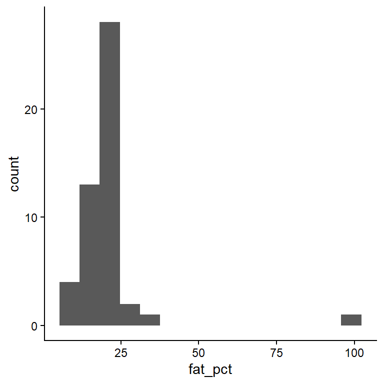

Figure 1.12: Histogram of fat percentage.

You should have spotted a potential outlier. Data entry errors are common, and a check against the original data sheet shows that the decimal was typed in the wrong place. The following code helps you locate the error.

which(scallop_df$fat_pct > 50) # which() returns the indexes

[1] 36

scallop_df$fat_pct[35:37] # row 36 is 99.0, but should be 9.90

[1] 22.8 99.0 12.9

scallop_df <- scallop_df[, c(1, 1)] # duplicate column
names(scallop_df) <- c("fat_pct_orig", "fat_pct_corr")
head(scallop_df, 2)

# A tibble: 2 × 2
  fat_pct_orig fat_pct_corr
         <dbl>        <dbl>
1         22.5         22.5
2         24.1         24.1

# there are many ways to 'fix' the outlier in R.
# You need to correct the outlier in row 36 of column 'fat_pct_corr'
scallop_df$fat_pct_corr[36] <- 9.9
which(scallop_df$fat_pct_corr > 90) 
# integer(0) - this means that no elements in fat_pct_corr contain values >90

Now summarise scallop_df using some of the methods above.

Q. 1.15

Create a histogram for the corrected column. How does it differ from the original column with the error?

Q. 1.16

Calculate mean, variance, median, interquartile range, minimum, maximum and range for both fat_pct_orig and fat_pct_corr.

Q. 1.17

Suppose the outlier was even bigger (i.e. your typo was even worse). Adjust your data, multiplying the erroneous data item by 10; copy the fat_pct_orig column and change row 36 to 999.

Q. 1.18

Calculate the same summary statistics.

Q. 1.19

Which measures of central tendency and variability are most ‘robust’ against this outlier?

Or look individually instead of calculating many metrics at once with tidyverse functions:

summary(scallop_df$fat_pct_corr)

   Min. 1st Qu.  Median    Mean 3rd Qu.    Max. 
   8.50   16.90   20.60   19.56   22.50   32.50

var(scallop_df$fat_pct_corr)

[1] 22.79836

IQR(scallop_df$fat_pct_corr)

[1] 5.6

R is excellent at generating well formatted tables such as shown in Table 1.1. What is missing from from this table?

Table 1.1: Summary statistics with and without an outlier. Note which summary stats are most influenced by the outlier.

Column	Mean	Median	Standard deviation	Range	Interquartile range
fat_pct_corr	19.6	20.6	4.77	24.0	5.6
fat_pct_orig	21.4	20.6	12.20	90.5	5.3

Q. 1.20

How would the patterns seen in Table 1.1 influence your choice if you were required to summarise data that you thought might contain values that could be erroneous? Consider how each metric is influenced by the data distribution and by outliers.

Let’s load a dataset that gives the length of hake across three years of sampling.

hake_df <- read_excel("data/H2SMS_practicalData.xlsx", sheet="Hake")
str(hake_df) # once again, column names made for excel rather than R

tibble [499 × 2] (S3: tbl_df/tbl/data.frame)
 $ Year            : num [1:499] 1 1 1 1 1 1 1 1 1 1 ...
 $ Hake length (mm): num [1:499] 190 219 181 148 206 204 168 197 178 211 ...

Q. 1.21

What type of variable is length?

Q. 1.22

Select an appropriate graphical method and display these data.

Hint: ggplot(..., aes(..., group=Year)) + geom_boxplot()

Q. 1.23

In your own time, summarise the hake data by year using the tidyverse functions you used above with the InsectSprays data.

hake_df$Year <- as.factor(hake_df$Year) # Treat as categorical, not numeric
names(hake_df) <- c("Year", "Length") # simplify the column names

Table 1.2: Summary of hake data.

Year	Mean length (cm)
1	201.8
2	497.0
3	988.9

The following ‘settling velocity’ data relates to the settling velocity of salmon faecal material. Shona Magill generated these data.

fishPoo_df <- read_excel("data/H2SMS_practicalData.xlsx", sheet="Settling velocity")
str(fishPoo_df)

tibble [200 × 1] (S3: tbl_df/tbl/data.frame)
 $ Settling velocity (mm s-1): num [1:200] 2.06 1.03 1.56 1.88 1.16 0.76 1.26 1.13 1.23 1.31 ...

Q. 1.24

Produce a histogram of the settling velocity. Is it left or right skewed?

Q. 1.25

Which measures of central tendency and variability are most appropriate?

Q. 1.26

Considering the distribution, is the mean or median larger?

Q. 1.27

Generate a new column of the log-transformed settling velocity data and plot these data.

Q. 1.28

What measures of central tendency and variability could be applied to the log-transformed data? Selecting the preferable metrics for a dataset is not necessarily straightforward.

Table 1.3 gives some indication of what issues you might consider.

Table 1.3: Appropriate measures of central tendency and variability according to the underlying data distribution.

Data distribution	Central tendency metric	Variability metric
Continuous, unimodal, symmetric	Mean	Variance or sd
Continuous, skewed	Median	Interquartile range
Continuous, multimodal	None; state modes	None; summarise by group
Discontinuous	None; data-dependent	Range?

1.5 Conclusions

Visualizing and summarising data are the critical first steps in the data analysis and reporting workflow. We use graphical methods to firstly explore our own data. Once we have made sense of it we select the most appropriate method to convey that understanding to our readers. We may help that communication by summarising data in the most appropriate way taking into account the distribution of the data and the presence of outliers.